All of old.
Nothing else ever.
Ever tried. Ever failed.
No matter.
Try again.
Fail again.
Fail better.
This is a quote from Worstward Ho by Samuel Beckett – a poem as impenetrable and opaque as my post on quantization. There is a version of Beckett’s poem with explanations, so I try again, too!
I stated that the description of a bunch of particles (think: gas in a box) naturally invokes the introduction of a hyperspace having twice as many dimensions as the number of those particles.
But it was obviously not obvious why we need those many dimensions. You have asked:
Why do we need additional dimensions for each particle? Can’t they live in the same space?
Why does the collection of the states of all possible systems occupy a patch in 1026 dimensional phase space?
These are nearly the same questions.
I start from a non-physics example this time, because I believe this might convey the motivation for introducing these dimensions better.
These dimensions are not at all related to hidden, compactified, extra large dimensions you might have read about in popular physics books on string theory and cosmology. They are not tangible dimensions in the sense we could feel them – even if we weren’t like those infamous ants living on the inflating balloon.
In Austria we recently had parliamentary elections. This is the distribution of seats in parliament – equivalent to these numbers:

SPÖ (52)
ÖVP (47)
FPÖ (40)
Grüne (24)
Team Stronach (11)
NEOS (9)
Using grand physics-inspired language I call that ordered collection of numbers: Austria’s Political State Vector.
These are six numbers thus this is a vector in a 6-dimensional Political State Space.
Before the elections websites consolidating and analyzing different polls have been more popular than ever. (There was a website run by physicist now working in finance.)
I can only display two of 6 dimensions in a plane, so the two axes represent any of those 6 dimensions. The final political state is represented by a single point in this space – the tip of an arrow:

After the elections we know the political state vector with certainty – that is: a probability of 1.
Before the elections different polls constituted different possible state vectors – each associated with a probability lower than 1. I indicate probabilities by different hues of red:

Each points represents a different state the system may finally settle in. Since the polls are hopefully meaningful and voters not too irrational points are not scattered randomly in space but rather close to each other.
Now imagine millions of polls – such as citizens’ political opinions tracked every millisecond by directly wiretapping their brains. This would result in millions of points, all close to each other. Not looking too closely, this is a blurred patch or spot – a fairly confined region of space covered with points that seems to merge into a continuous distribution.

Watching the development of this red patch over time lets us speculate on the law underlying its dynamics – deriving a trend from the dynamics of voters’ opinions.
It is like figuring out the dynamics of a moving and transforming piece of jelly.
Back to Physics
Statistical mechanics is similar, just the numbers of dimensions are much bigger.
In order to describe what each molecule of gas in a room does, we need 6 numbers per molecules – 3 for its spatial coordinates, and 3 for its velocity.
Each particle lives in the same real space where particles wiggle and bump into each other. All those additional dimensions only emerge because we want to find a mathematical representation where each potential system state shows up as a single dot – tagged with a certain probability. As in politics!
We stuff all positions and velocities of particles into an enormous state vector – one ordered collection with about 1026 different numbers corresponds to a single dot in hyperspace.
The overall goal in statistical mechanics is to calculate something we are really interested in – such as temperature of a gas. We aim at calculating probabilities for different states!
We don’t want to look to closely: We might want to compare what happens if if we start from a configuration with all molecules concentrated in a corner of the room with another one consisting of molecules everywhere in the room. But we don’t need to know where each molecule is exactly. Joseph Nebus has given an interesting example related his numerical calculation of the behavior of a car’s shock absorbers:
But what’s interesting isn’t the exact solution of the exact problem for a particular set of starting conditions. When your car goes over a bump, you’re interested in what the behavior is: is there a sudden bounce and a slide back to normal? Does the car wobble for a short while? Does it wobble for a long while? What’s the behavior?
You have asked me for giving you the equations. I will try my best and keep the intro paragraphs of this post in mind.
What do we know and what do we want to calculate?
We are interested in how that patch moves and is transformed – that is probability (the hue of red) as a function of the positions and momenta of all particles. This is a function of 1026 variables, usually called a distribution function or a density.
We know anything about the system, that is the forces at play. Knowing forces is equivalent to knowing the total energy of a system as a function of any system configuration – if you know the gravitational force a planet exerts than you know gravitational energy.
You could consider the total energy of a system the infamous formula in science fiction movies that spies copy from the computer in the secret laboratories to their USB sticks: If you know how to calculate the total energy as a function of the positions and momenta of all particles – you literally rule the world for the system under consideration.
Hyper-Planes
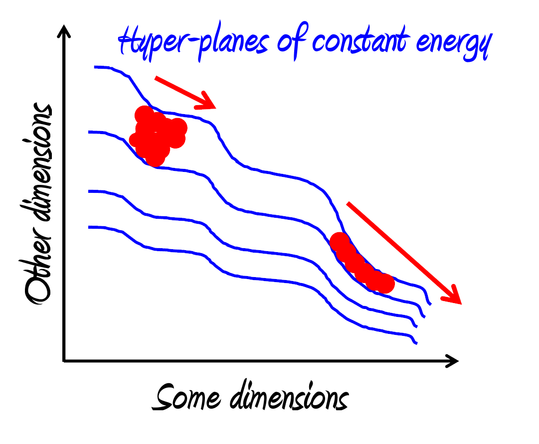
If we know this energy ‘world function’ we could attach a number to each point in hyperspace that indicate energy, or we could draw the hyper-planes of constant energies – equivalent of isoclines in a map.
The dimension of the hyperplane is the dimension of the hyperspace minus one, just as the familiar 2D planes floating through 3D space.
If energy changes more rapidly with varying particle positions and momenta hyper-planes get closer to each other:

Incompressible Jelly
We are still in a classical world. The equations of motions of hyper-jelly are another way to restate Newton’s equations of motion. You start with writing down Force = mass x accelerating for each particle (1026 times), rearrange these equations by using those huge state vectors just introduced – and you end up with an equation describing the time evolution of the red patch.
I picked the jelly metaphor deliberately as it turns out that hyper-jelly acts as an incompressible fluid. Jelly cannot be destroyed or created. If you try to squeeze it in between two planes it will just flow faster. This really follows from Newton’s law or the conservation of energy!

It might appear complicated to turn something as (seemingly) comprehensible as Newton’s law into that formalism. But that weird way of watching the time evolution of the red patch makes it actually easier to calculate what really matters!
Anything that changes in the real world – the time evolution of any quantity we can measure – is expressed via the time evolution of hyper-jelly.
The Liouville equation puts this into math.
As Richard Feynman once noted wisely (Physics Lectures, Vol.2, Ch. 25), I could put all fundamental equations into a big matrix of equations which I then call the Unwordliness, further denoted as U. Then I can unify them again as
U = 0
What I do here is not that obscure but I use some pseudo-code to obscure the most intimidating math. I do now appreciate science writers who state We use a mathematical crank that turns X into Y – despite or because they know exactly what they are talking about.
For every point in hyperspace the Liouville equation states:
(Rate of change of some interesting physical property in time) =
(Some mathematical machinery entangling spatial variations in system’s energy and spatial variations in ‘some property’)
Spatial variations in the system’s energy can be translated to the distance of those isoclines – this is exactly what Newton’s translates into! (In addition we apply the chain rule in vector calculus).
The mathematical crank is indicated using most innocent brackets, so the right-hand side reads:
{Energy function, interesting property function}
Quantization finally seems to be deceptively simple – the quantum equivalent looks very similar, with the right-hand side proportional to
[Energy function, interesting property function]
The main difference is in the brackets – square versus curly: We consider phase space so any function and changes thereof is calculated in phase space co-ordinates – positions and momenta of particles. These cannot be measured or calculated in quantum mechanics with certainty at the same time.
In a related way the exact order of operations does matter in quantum physics – whereas the classical counterparts are commutative operations. The square bracket versus the angle bracket is where these non-commutative operations are added – as additional constraints to classical theory.
I think I have reached my – current – personal limits in explaining this, while still not turning this blog into in a vector calculus lecture. Probably this stuff is usually not popularized for a reason.
My next post will focus on quantum fields again – and I try to make each post as self-consistent anyway.


Leave a Reply